ParlLawSpeech Tutorials

Tutorial 1:
How much are legislatives bills debated on the plenary floor?

Members of parliament (MPs) fulfill important representative and communicative functions in linking societal preferences to legislative decisions. They need to demonstrate that they represent their constituencies in decision-making and they are crucial for communicating and assessing the laws that are discussed and decided in parliament. Plenary debates offer a useful and usually publicly very visible forum to live up to these ideals.

But given the myriad of legislation that modern parliaments have to process, one may reasonably ask: How many bills actually reach the open debates on the plenary floor? How much plenary attention do bills actually receive?

One basic indicator to systematically approach these questions would be the average number of speeches per bill tabled in parliament. This indicator, however, requires data linkage: one first needs to know which speech covers which bill.

During our data collection we have carefully inspected, coded, and ultimately linked the agenda information on plenary debates in parliamentary archives with the meta information in document databases of bills and adopted laws. The ParlLawSpeech files thus can provide exactly this link through the unique procedure_ID variable. In this example, we exploit and illustrate this in the example of the Hrvatski sabor, the unicameral legislature of the Republic of Croatia (HR), which our data covers throughout the 2003-2020 period.

So let’s first load the respective speech data set (we are assuming that you have PLS country folders and files in you current working directory - if not you will have to adapt the path to the files here).

speeches <- read_rds(here("Croatia", "Corpus_speeches_croatia.RDS"))

We then aggregate these data along the procedure_ID variable and count how many speeches we have for each value on this variable.

speechesPerBill <- speeches %>% # Copy of the speeches data set ...
  group_by(procedure_ID) %>% # ... group by bill-specific ID ...
  summarize(nspeeches = n()) %>% # ... sumarise by counting the number of obs (=speeches) per ID ...
  filter(procedure_ID != "") %>% # ... and ignore speeches that did not cover specific bills.
  ungroup() %>% 
  arrange(desc(nspeeches)) # Sort bills in descending order by number of corresponding speeches

kable(head(speechesPerBill))

Nice. But as we have started from the speech data set, we now only ‘see’ those bills that were actually covered by at least one speech on the plenary floor. We thus might miss bills that have not have been debated at all. With ParlLawSpeech we can check this with the help of the bills data set provided for each country.

Let’s load the respective Croatian data and compare it to the aggregate speeches-per-bill data we have just created above.

bills <- read_rds(here("Croatia", "Corpus_bills_croatia.RDS")) %>% 
  select(procedure_ID, title_bill) %>% 
  unique() # remove duplicates

nrow(bills)

## [1] 3676

nrow(speechesPerBill)

## [1] 2879

We see that the bills data set contains 797 rows more than we have retrieved from the speeches data set, suggesting that many bills actually never reached the plenary floor.

Before digging into this further, there is a second second issue to note: parliaments often discuss several bills together in one debate. In such instances our data contain multiple entries in the procedure_ID variable. Look at one example:

speechesPerBill$procedure_ID[13]

## [1] "P.Z.452_09, P.Z.453_09, P.Z.454_09"

This debate apparently covered three bills (with consecutive numbering along the conventions of the Croatian parliament). From the meta data alone, unfortunately, it is impossible to say whether an individual speech in this particular debate referred only to one, to two, or to all of these bills (which are probably closely related anyway). For the purposes here, we attribute each speech to each of the respective bills in this debate (one alternative assumption may be that only one third of the speeches can be attributed to each bill, but let’s keep it simple for now…).

On this basis, we can now traverse through our full bill data for Croatia and look up the number of speeches that each bill has received in our earlier aggregation of the speech data set.

bills$nspeeches <- 0 # Set the number of speeches per bill initially to 0

for (i in 1:nrow(bills)) { # Loop through all bills ...
  
  # ... look up in which row of the speechesPerBill aggregation the bill id occurs ...
  row <- which(str_detect(fixed(speechesPerBill$procedure_ID), bills$procedure_ID[i]))
  
  if (length(row)>0) { # ... and if the bill was debated on the plenary floor ...
    
    # ...  store the number of respective speeches in the bills data
    bills$nspeeches[i] <- speechesPerBill$nspeeches[row[1]]
  }
}

bills <- bills %>% 
  arrange(desc(nspeeches)) # Sort the data in descending number of speeches per bill

This provides the final number of plenary speeches per each individual bill that was tabled in the Croatian parliament between 2003 and 2020. What does this information say about our initial questions? Have a look at the basic summary statistics first.

summary(bills$nspeeches)

##    Min. 1st Qu.  Median    Mean 3rd Qu.    Max. 
##    0.00   14.00   39.00   88.76  106.25 2253.00

We get a first answer: In the Croatian parliament, an average legislative bill is debated in 88.76 speeches. Quite a bit of debate, indeed.

But wait, the minimum value is 0! As suspected there are also bills that are never debated on the plenary floor. Let’s have a look at their overall share:

mean(bills$nspeeches == 0)*100

## [1] 7.725789

This provides a second answer: about 8 per cent of bills are actually never debated in the plenary of the Croation parliament …

Moreover, the summary statistics above suggest that the distribution of speeches per bill is rather skewed. The median value is ‘only’ 39 speeches per bill but the maximum goes up to 2,253 speeches. Let’s visualize this distribution.

ggplot(bills, aes(x=nspeeches))+
  geom_histogram(bins = 60, fill = "#0063a6", alpha = .8)+
  labs(title = "Plenary speeches per legislative bill in the Croatian Hrvatski sabor, 2003-2020",
       x = "Number of speeches per bill (binned)",
       y = "Frequency")+
  theme_bw()+
  theme(
    plot.title = element_text(face = "bold.italic"),
    strip.background = element_rect(fill= NA),
    panel.grid.minor = element_blank())

Plenary attention to individual bills is actually very skewed. In other words, speeches in the plenary debates concentrate on a few bills. Of the 3,676 bills, only 1,590 receive more than 50 speeches (in a parliament that consists of 151 seats at the time of writing).

Moreover, a few bills receive extraordinary plenary attention. As we have sorted the data set in descending order above, we can readily look at the bill that received the most MP speeches in the Croatian Hrvatski sabor between 2003 and 2020.

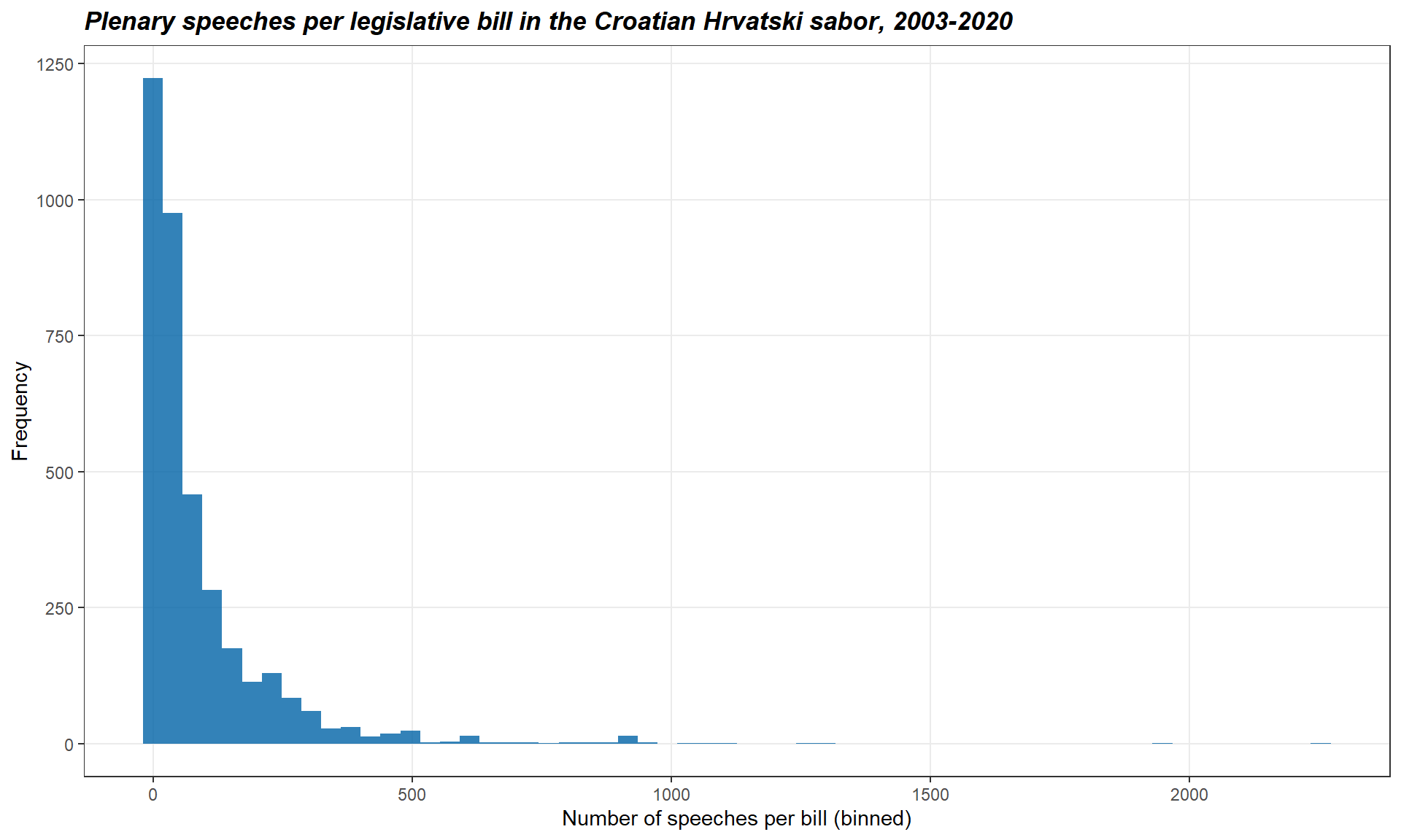
kable(bills[1,])

On two days in early 2019, the “Proposal of the law on the financing of political activities, election campaigns and referendums” (with a little help by Google Translate …) was debated in 2,253 MP speeches. Party finances seem to be a hot topic for MPs …

Of course, much more has to be done to turn this initial demonstration into a substantially meaningful analysis. But already this simple example shows that the linkages between different types of parliamentary documents generate systematic insights into the parliamentary process that were not visible with such precision before.

From here, more in-depth analysis could, for example, classify the text in the bill titles to analyse whether plenary attention is systematically biased for or against certain topics. Or you might be interested whether and to what extent the concentration of plenary debates on few specific bills observed for the Croatian parliament is different from other countries. Go ahead, ParlLawSpeech offers data to pursue such questions …

Tutorial 2:
How much do legislative bills change during the parliamentary process?

One often-heard criticism of modern parliaments is that they are dominated by the executive: parliamentary majorities are accused to just rubber-stamp the legislative bills that governments serve them rather than actually shaping the content of binding law. To what extent does this hold true? How much do legislative bills actually change during the parliamentary process?

Again such questions require data linkage, here specifically links of tabled bills and the finally adopted laws. Such questions also require data along which these pairs of bills and adopted laws can be systematically compared. The full-text vectors of legislative documents in ParlLawSpeech encapsulate lots of information useful to that end.

To illustrate how to exploit these ParlLawSpeech features, this tutorial resorts to the data for the Spanish Congreso de los Diputados in the 1996-2023 period.

Let’s load these and join the relevant information for bills and adopted laws along the procedure_ID variable.

# Load bills data for Spain,
# Select relevant variables and mark government-sponsored bills
bills <- read_rds(here("Spain", "Corpus_bills_spain.RDS")) %>% 
  select(procedure_ID, title_bill, bill_text, initiator) %>% 
  mutate(sponsor = ifelse(initiator == "Gobierno",
                          "Government", "Other") %>% 
           factor(levels = c("Government", "Other"))) %>% 
  select(-initiator) %>% 
  filter(!is.na(sponsor))

# Law data for Spain
laws <- read_rds(here("Spain", "Corpus_laws_spain.RDS")) %>% 
  select(procedure_ID, title_law, law_text)

# Combine bill and law information
comp <- bills %>% 
  left_join(laws %>% 
              select(procedure_ID, title_law, law_text), 
            by = "procedure_ID")

This linked data initially provides us information on how many bills actually turned into binding law - as indicated by the presence or absence of a respective law text. The ParlLawSpeech data furthermore provide information on who tabled the bill in the first place.

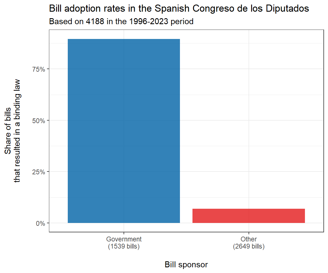
Pulling this together allows us to visualize the success rates of government-sponsored bills vs. those of bills tabled by other actors (typically individual partisan factions in the Congreso or autonomous Spanish regions).

# Calculate bill adoption rates
adoptionrates <- comp %>% # Calculate adoption rates ...
  group_by(sponsor) %>% # ... by bill sponsor
  summarise(nbills = n(), # Number of bills
            adoption.rate = 1 - mean(is.na(law_text))) %>% # Absence of law text as non-adopted
  ungroup() %>% 
  mutate(sponsor2 = paste0(sponsor, "\n(", nbills, " bills)"))

# Plot these data
ggplot(adoptionrates, aes(y = adoption.rate, x = sponsor2, fill = sponsor2))+
  geom_col(alpha = .8)+
  scale_fill_manual(values = c("#0063a6", "#e41a1c"))+
  scale_y_continuous(labels = scales::percent)+
  labs(title = "Bill adoption rates in the Spanish Congreso de los Diputados",
       subtitle = paste0("Based on ", sum(adoptionrates$nbills), " in the 1996-2023 period"),
       x = " \nBill sponsor",
       y = "Share of bills\nthat resulted in a binding law\n ")+
  theme_bw()+
  theme(legend.position = "none")

We clearly find that the likelihood that a bill is adopted by the Spanish lower house is significantly higher when it comes from the government (89.6% as opposed to 6.95%). This is initially consistent with the ‘executive dominance’ criticism.

But, of course, that does not have to mean that parliament adopts these laws exactly as the government has proposed them. To answer how much bills are changed during the parliamentary process we have to systematically compare their content.

For such a comparison, the full-text vectors that ParlLawSpeech offers come in handy. We first reduce the data to procedures for which both a bill and an adopted law text are available.

pairs <- comp %>% 
  filter(!is.na(bill_text) & !is.na(law_text))

Before comparing the text pairs, one disclaimer is in order. As noted above, the full-text vectors in ParlLawSpeech equal the way in which the respective source archive provides them so as to give researchers maximum freedom in selecting, cleaning, and pre-processing the text data in ways that fit the text analysis of interest. Inversely, of course, this means that researchers will often need to clean the texts in ways that suits their planned analysis. We thus recommend that ParlLawSpeech users carefully inspect and acquaint themselves in great detail with the structure of the provided texts before plugging them into automated text analysis algorithms (recall: garbage in -> garbage out).

With the code below, for example, users can export random examples to local files, which can then be inspected with standard text editors (we recommend Notepad++, for example).

# Pick random row
i <- sample(1:nrow(pairs), 1)
i

# Meta-info on picked example
pairs$title_bill[i]
pairs$title_law[i]
pairs$procedure_ID[i]

# Export bill and law text to local files for inspection
writeLines(pairs$bill_text[i], "BillExample.txt")
writeLines(pairs$law_text[i], "LawExample.txt")

For our interest in bill-to-law change for this tutorial, we want to compare only the legal substance of the documents, that is the legal articles that actually stipulate the binding rules in a law. In other words, we want to remove all recitals, preambles, justifications, appendices and other boilerplate (which might be relevant for other analyses, of course).

To achieve this we inspected and cross-checked numerous examples and noted recurring patterns that would help us to isolate the text bits of interest. We then generalized these patterns to regular expressions which we then match across the texts with the functions of the stringR package (contained in the tidyverse package we have loaded above).

This is a time-consuming, but often necessary step. For learning how to use regular expressions in R we can recommend this resource. For developing specific regular expressions and for testing them with exemplary texts, sandbox tools such as regexr.com are usually also very helpful.

Such pre-processing steps should always be well documented and usually also very extensively validated. For our purposes here we use the following (admittedly somewhat crude) text cleaning steps to cut the raw texts before and after their legal substance:

# Cleaning bill texts
pairs$bill_text_redux <- 
  # Copy of raw bill text
  pairs$bill_text %>% 
  # Missing white spaces after punctuation
  str_replace_all("(\\.|,|;)([A-Z])", "\\1 \\2") %>%  
  # Reduce multiple consecutive whitespaces to one regular whitespace
  str_replace_all("\\s+", " ") %>% 
  # Remove everything before the legal text begins
  # "Article 1" heading (only valid if followed by a capitalized word)
  str_remove(regex("^.*? PREÁMBULO", 
                   ignore_case = F)) %>% # Remove everything up to the preamble, needed in case law text has an article index
  str_replace(regex("^.*? (art(í|i)culo)\\s+(1|(u|ú)nico|pr(í|i)mero)(\\.|:| )\\s*([A-ZÁÉÍÓÚ])", 
                    ignore_case = T), "Artículo 1. X") %>% 
  # Remove Appendices
  # str_remove("\\.\\s+ANEXO\\s+([0-9]|I).*") %>%
  str_remove(regex("\\s+ANEXO\\s+([0-9]|I)\\s.*?$", ignore_case = F)) %>%
  # Remove HTML and other gibberish
  str_remove_all("<.*?>") %>%  
  str_remove_all("\\[\\*.*?\\*\\]") %>% # Some strange table / page formatting 
  # Final, non-substantial edits
  str_replace_all("[[:punct:]]", " ") %>% 
  str_replace_all("\\s+", " ") %>% 
  str_trim() %>% 
  tolower()

# Cleaning law texts
pairs$law_text_redux <- 
  # Copy of raw law text
  pairs$law_text %>% 
  # Missing whitespaces after punctuation
  str_replace_all("(\\.|,|;)([A-Z])", "\\1 \\2") %>% 
  # Reduce multiple consecutive whitespaces to one regular whitespace
  str_replace_all("\\s+", " ") %>% 
  # Remove everything before the legal text begins
  # "Article 1" heading (only valid if followed by a capitalized word)
  str_remove(regex("^.*? PREÁMBULO", 
                    ignore_case = F)) %>% # Remove everything up to the preamble, needed in case law text has an article index
  str_replace(regex("^.*? (art(í|i)culo)\\s+(1|(u|ú)nico|pr(í|i)mero)(\\.|:| )\\s*([A-ZÁÉÍÓÚ])", 
                    ignore_case = T), "Artículo 1. X") %>% 
  # Remove Appendices
  # str_remove("\\.\\s+ANEXO\\s+([0-9]|I).*") %>%
  str_remove(regex("\\s+ANEXO\\s+([0-9]|I)\\s.*?$", ignore_case = F)) %>%
  # Remove HTML and other gibberish
  str_remove_all("<.*?>") %>%  
  str_remove_all("\\[\\*.*?\\*\\]") %>% # Some strange table / page formatting 
  # Final, non-substantial edits
  str_replace_all("[[:punct:]]", " ") %>% 
  str_replace_all("\\s+", " ") %>% 
  str_trim() %>% 
  tolower()

# Re-check examples
# i <- sample(1:nrow(pairs), 1)
# i
# writeLines(pairs$bill_text_redux[i], "BillExample.txt")
# writeLines(pairs$law_text_redux[i], "LawExample.txt")

# Keep only bills that actually draft legal text
# (in a few instances Spnish bills just describe rather than actually propose legal text)
pairs <- pairs %>% 
  filter(str_detect(bill_text_redux, "artículo 1 x"))

# Remove everything after the final 'entry into force' article in each law text/proposal
pairs$bill_text_redux <-
  pairs$bill_text_redux %>% 
  str_remove("entrará en vigor (a|e)l día siguiente (al ){0,1}de su publicación en el boletín oficial del estado.*?$")
pairs$law_text_redux <-
  pairs$law_text_redux %>% 
  str_remove("entrará en vigor (a|e)l día siguiente (al ){0,1}de su publicación en el boletín oficial del estado.*?$")

# Filter case with apparent archive errors
pairs <- pairs %>% 
  filter(procedure_ID != "121/000065 Leg.6") %>% # Bill and law title don't match
  filter(procedure_ID != "121/000012 Leg.7") %>% # Bill and law title don't match
  filter(procedure_ID != "121/000033 Leg.8") # Bill text doesn't match title

# Store intermediate results (so to avoid having to repeat the above - this takes some time)
write_rds(pairs, here("TutorialOutputs", "ES_CleanedBillsAndLaws.RDS"))

Having reduced the bill and law text to their legal core, we can now compare them pair by pair.

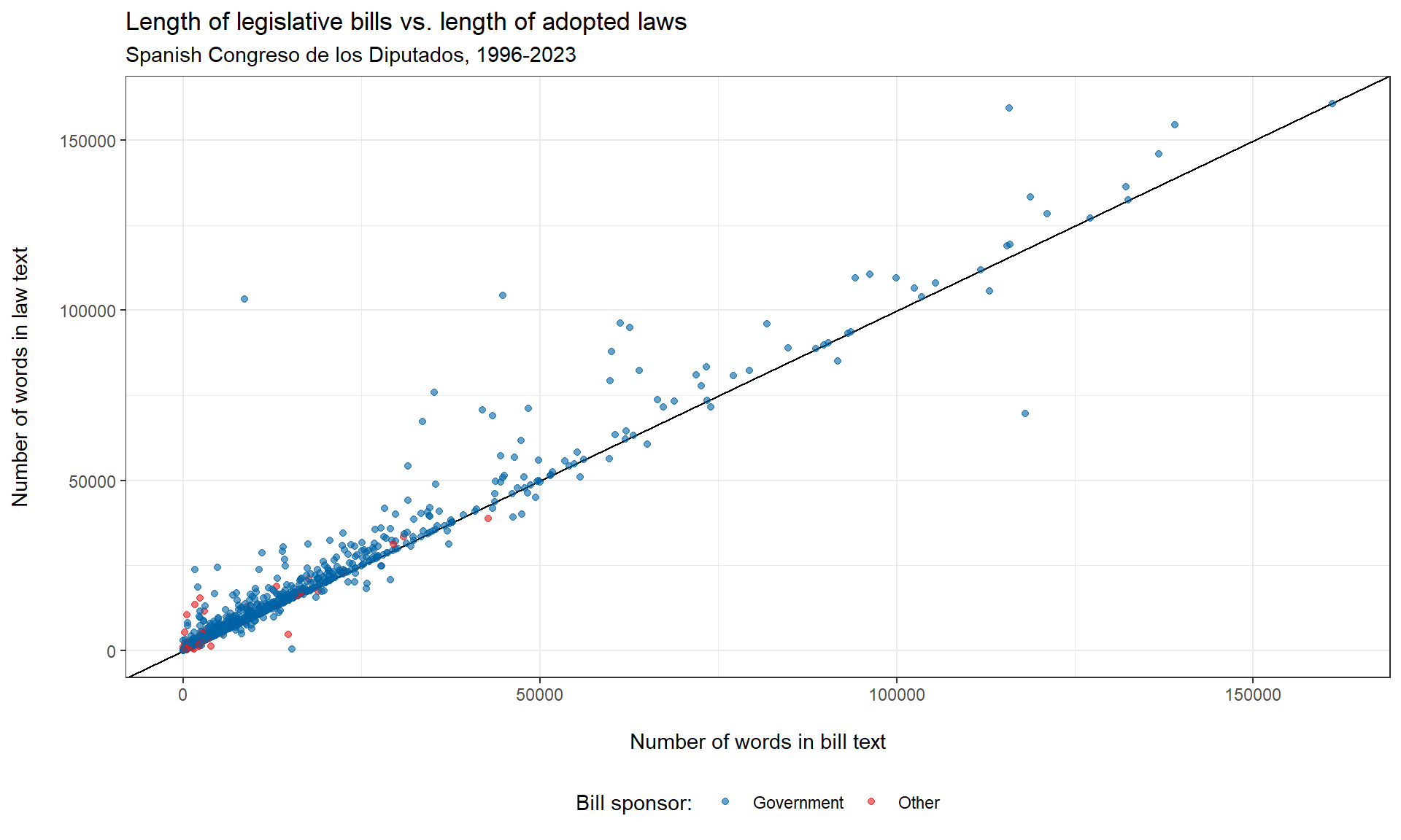
An initial, very simple indicator for legal change during the parliamentary process is the amount of words that are added or removed from the bill before it is adopted as law.

In the following steps we thus count the number of words in each text (again using a regular expression) and then plot the length of bills against the length of the respective laws.

# Reloaded the cleaned texts
pairs <- read_rds(here("TutorialOutputs", "ES_CleanedBillsAndLaws.RDS"))

# Word counts
pairs$billlength <- str_count(pairs$bill_text_redux, "\\w+")
pairs$lawlength <- str_count(pairs$law_text_redux, "\\w+")
pairs$lengthdiff <- pairs$lawlength - pairs$billlength

# Plot length differences
ggplot(pairs ,aes(x = billlength, y = lawlength, color = sponsor))+
  geom_abline(intercept = 0, slope = 1)+ # 45° line indicating identical word counts of bills and laws
  geom_point(alpha = .6)+
  # geom_smooth(method = "loess")+
  scale_color_manual(values = c("#0063a6", "#e41a1c"))+
  labs(title = "Length of legislative bills vs. length of adopted laws",
       subtitle = "Spanish Congreso de los Diputados, 1996-2023", 
       x = " \nNumber of words in bill text",
       y = "Number of words in law text\n ",
       color = "Bill sponsor: ")+
  theme_bw()+
  theme(legend.position = "bottom")

Apparently the majority of legislative procedures clusters around the 45° degree line which indicates that the length of the finally adopted law largely equals the length of the initial bill. But we also note quite a number of deviating cases mostly significantly above the 45° line.

In other words, the word count of bills changes often only very little during the parliamentary process in the Spanish Congreso, but when it does the resulting laws tend to become longer than the initial bill.

Of course, an apparently by-and-large stable word count may still mask significant and political change depending on whether and which words are added, removed or replaced. Such within-text change can be aggregated by comparing word frequency matrices and normalizing their overlap, for example by the Cosine similarity measure.

But not only the differing frequency of words but also their order can matter a great deal in politics. Consider the following hypothetical examples:

• We prioritize the environment over the economy!
  
• We prioritize the economy over the environment!

Both sentences have the same length and they also contain exactly the same words (the Cosine similarity of their word frequency matrix equals 1). But in terms of political meaning, they are arguably very different.

One approach to retrieve a frequency-based similarity measure that is at least somewhat sensitive to word order is to tokenize (= split) the texts not into individual words but into sequences of consecutive words (so-called ngrams). Tokenizing the above examples into overlapping bigrams (sequences of two consecutive words), for example, would look like this:

• [We prioritize] [prioritize the] [the environment] [environment over] [over the] [the economy]
• [We prioritize] [prioritize the] [the economy] [economy over] [over the] [the environment]

Of the six bigrams in each example, only five occur in both texts - resulting in a lower cosine similarity of .83. The longer the ngrams that we split the text into, the more sensitive our similarity measure becomes to changes in word order.

Let’s apply these ideas to our text data from the Spanish Congreso. The following code traverses through all 1,534 bill/law pairs and uses functions from the quanteda R package to split each text into overlapping 5-grams, to store their frequency in a matrix, and to then calculate the Cosine similarity for each each bill/law pair.

# Empty traget variable
pairs$cosine5 <- NA

# Loop through text pairs,
# get frequency matrix of 5-grams for respective bill and law
# calculate cosine similarity of both matrixes
for (i in 1:nrow(pairs)) {
  
  a.mat <- corpus(pairs$bill_text_redux[i]) %>% 
    tokens() %>% tokens_ngrams(n = 5) %>% 
    dfm() %>% dfm_weight("prop")
  
  b.mat <- corpus(pairs$law_text_redux[i]) %>% 
    tokens() %>% tokens_ngrams(n = 5) %>% 
    dfm() %>% dfm_weight("prop")
  
  pairs$cosine5[i] <- textstat_simil(a.mat, b.mat, 
                                     method = "cosine", 
                                     margin = "documents")[1]
}

# Store intermediate result
# So as not having to run this again and again (a little bit of computation is involved here...)
write_rds(pairs %>% select(procedure_ID, sponsor, cosine5), here("TutorialOutputs", "ES_BillLawCosine.RDS"))

Based on 5-word sequences, this measure gives us a relative estimate of the similarity between the bill and the finally adopted law.

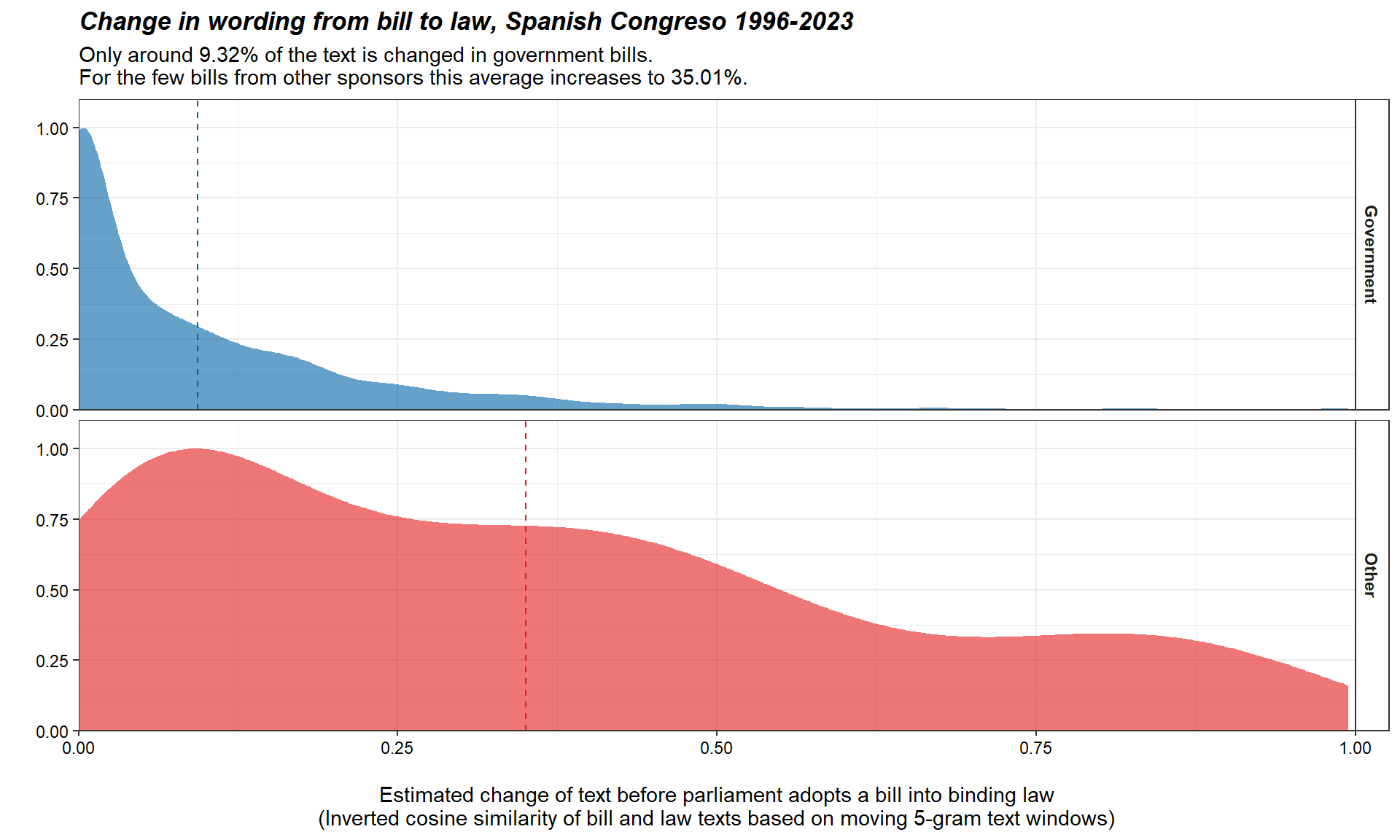
Inverting it accordingly allows us to plot legislative change during the parliamentary process across the 1,534 bills/law pairs for the 1996-2023 period we observe here.

# Reload the Cosine similarity data
pairs <- read_rds(here("TutorialOutputs", "ES_BillLawCosine.RDS"))

# Invert cosine similarity to express change rather than similarity
pairs$cosine5inv <- 1 - pairs$cosine5

# Calculate average text changes
avchange <- pairs %>% 
  group_by(sponsor) %>% 
  summarise(avchange = mean(cosine5inv))

# Plot full distribution
ggplot(pairs,aes(x = cosine5inv,  color = sponsor, fill = sponsor, ..scaled..))+
  geom_density(alpha = .6, color = NA)+
  facet_wrap(~sponsor, nrow = 2,
             strip.position = "right")+
  geom_vline(data=filter(pairs, sponsor=="Government"), aes(xintercept= mean(cosine5inv)), colour="#0063a6", linetype = "dashed")+
  geom_vline(data=filter(pairs, sponsor=="Other"), aes(xintercept= mean(cosine5inv)), colour="#e41a1c", linetype = "dashed")+
  # geom_density_ridges(alpha = .6, scale = 1.2, rel_min_height = 0.001)+
  # stat_density_ridges(quantile_lines = TRUE, alpha = .6, scale = 1.2, rel_min_height = 0.001)+
  labs(title = "Change in wording from bill to law, Spanish Congreso 1996-2023",
       subtitle = paste0("Only around ", 
                         round(avchange$avchange[avchange$sponsor == "Government"]*100,2) ,  
                         "% of the text is changed in government bills. \nFor the few bills from other sponsors this average increases to ",
                         round(avchange$avchange[avchange$sponsor == "Other"]*100,2),
                         "%."),
       x = " \nEstimated change of text before parliament adopts a bill into binding law\n(Inverted cosine similarity of bill and law texts based on moving 5-gram text windows)",
       y = " ")+
  scale_x_continuous(expand = c(0, 0))+
  scale_y_continuous(expand = expansion(mult = c(0, .1)))+
  scale_color_manual(values = c("#0063a6", "#e41a1c"))+
  scale_fill_manual(values = c("#0063a6", "#e41a1c"))+
  coord_cartesian(xlim = c(0, 1))+
  theme_bw()+
  theme(legend.position = "none",
        axis.text = element_text(color = "black"),
        strip.text = element_text(face = "bold"),
        strip.background = element_rect(fill= NA),
        plot.title = element_text(face = "bold.italic"))

This highlights that government bills actually change very little during the parliamentary process. On average (and based on comparing 5-gram sequences of words), only 9.32% of the text is changed in a government bill before parliament adopts it as law. Looking at the full distribution, moreover, suggests that this average is driven by a few outliers - the median government bill ‘experiences’ only 4.11% of textual change during processing in parliament.

In contrast, the few adopted bills tabled by other sponsors are changed much more significantly during the parliamentary process. On average, more than a third of the text of such bills is altered and the overall distribution across all such bills is much flatter than that for government-sponsored bills.

Again, this is a relatively quick analysis. Users wishing to push this further may invest in more careful pre-processing and especially look into minimum edit distance algorithms that have been recently successfully applied to study legislative change (e.g Cross and Hermanson, 2017, Rauh 2020). These tools can then be used to test theories about the legislative influence of parliaments in a comparative fashion, e.g. across specific bills, across different governments, or even across countries.

For now, however, also this comparatively simple example showcases the analytical potential in the availability of linked full-text data on the parliamentary process. What can you do with it?

Tutorial 3:
How does the debate on a specific bill differ from other debates?

In many instances analysts will be interested in whether and how the debate on one specific bill differs from typical behavior in the respective parliament. To illustrate such an application with the ParlLawSpeech data, this tutorial focuses on the legal framework for containing COVID-19 in Germany.

Specifically, we look at the third installment of the so-called ‘Law for the Protection of the Population in an Epidemic Situation of National Concern’ (‘Drittes Gesetz zum Schutz der Bevölkerung bei einer epidemischen Lage von nationaler Tragweite’) which was introduced to the German Bundestag on November 3 2020.

In a context of still growing infection rates, legal and political disputes on prior pandemic measures, and partially massive street protests, this bill aimed to regulate and to define the conditions under which the executive could enact partially far-reaching interventions such as lockdowns or prohibitions of rallies, amongst others.

In this context, the grand-coalition government (Merkel IV) aimed for a broad parliamentary debate that would ideally generate support of the proposed measures (which were formally tabled not by the government for that reason but by the faction leaders of the governing parties CDU/CSU and SPD). So how much plenary attention did the different parties in the German Bundestag devote to debating this law in comparison to others? And did the resulting debate actually transcend the typical government-opposition dynamics?

To approach these exemplary questions in a systematic manner, we first load the speech data set for the German Bundestag and filter it for meaningful comparison. Specifically, we include speeches that …

• were given during the Merkel IV government,
  
• were not given by the chair of the debate and were longer than five words (excluding merely organisational statements),
  
• addressed any legislative bill,
  
• and were given by a member of a political faction.

speeches <- read_rds(here("Germany", "Corpus_speeches_germany.RDS")) %>% 
  select(date, chair, speaker, party, text, procedure_ID) %>% 
  filter(date >= "2018-03-14" & date < "2021-12-08") %>% # Debates during the Merkel IV government
  filter(!chair) %>% # Drop organisational speeches from the chair
  filter(str_count(text, "\\w+") >= 5) %>% # Keep only speeches longer than 5 words 
  filter(procedure_ID != "") %>% # Keep only bill-specific debates | TO DO: encode as NA 
  filter(!is.na(party) & party != "fraktionslos") # Drop non-partisan speakers

To identify which of these 7,148 speeches address the bill we are interested in here, we initially load the bill data for Germany and also reduce it to all bills tabled during the Merkel IV government.

# Load the German bill data
bills <- read_rds(here("Germany", "Corpus_bills_germany.RDS")) %>% 
  select(procedure_ID, initiator, initiation_date, title_bill) %>% 
  filter(initiation_date >= ymd("2018-03-14") & initiation_date < ymd("2021-12-08"))

Knowing the German title of the proposed law and the initiation date, we can then retrieve the respective procedure_ID which provides the link to the relevant speeches.

billsOfInterest <- bills %>% 
  filter(str_detect(title_bill, "Schutz der Bevölkerung bei einer epidemischen Lage von nationaler Tragweite")) %>%   filter(initiation_date == ymd("2020-11-03"))
kable(billsOfInterest)

To assess the plenary attention to this bill (in comparison to all others under the Merkel IV government), we proxy bill-specific speaking time by the number of words that speakers from each faction uttered on each bill.

NumberOfWords <- 
  # Start from the speech data ...
  speeches %>% 
  # ... count number of words with a regular expression matching groups of so-called word characters
  # including upper and lower case charcters as well as numbers ...
  mutate(wordcount = str_count(text, "\\w+")) %>% 
  # ... group by bill and partisan faction ...
  group_by(procedure_ID, party) %>% 
  # ... and retrieve the sum of words spoken for each group ... #
  summarise(wordcount = sum(wordcount)) %>% 
  # ... mark the law of interest, using it's ID retrieved above ...
  mutate(covid = str_detect(procedure_ID, "19/23944/19")) %>%
  # ... and summarise across this law and all others ...
  group_by(covid, party) %>% 
  # .. along the mean number of words spoken and a bootstrapped confidence interval.
  summarise(ci = list(mean_cl_boot(wordcount) %>% 
                        rename(mean=y, lwr=ymin, upr=ymax))) %>% 
  unnest(cols = c(ci))

Then we provide more telling labels for the bill group variable. We also order the parties by their share of seats in the 19th German Bundestag as this should be be roughly proportional to their speaking time according to the Bundestag’s internal rules.

# Label debate
NumberOfWords$covid2 <-
  ifelse(NumberOfWords$covid == T,
         "on the third installment of the Infection Protection Act",
         "on all other bills debated during the Merkel IV government (average)") %>% 
  factor(levels = c("on all other bills debated during the Merkel IV government (average)", "on the third installment of the Infection Protection Act"))

# Order parties (by size of faction in 19th Bundestag)
NumberOfWords$party2 <- factor(NumberOfWords$party,
                                         levels = c("BÜNDNIS 90/DIE GRÜNEN", "DIE LINKE", "FDP", "AfD", "SPD", "CDU/CSU")) %>% 
  fct_rev()

This data then allows us to comparatively visualize the plenary attention that each party devoted to the third installment of the Infection Protection Act - in comparison to all other bills during the Merkel IV government.

# Plot number of speeches
ggplot(NumberOfWords, aes(x = party2, y = mean, ymin = lwr, ymax = upr, color = party2, fill = party2, group = covid2))+
  geom_linerange(position = position_dodge(width = .5))+
  geom_col(position = position_dodge(width = .5), width = .5, aes(alpha = covid2))+
  scale_color_manual(values = c("black", "#E3000F", "#3c9dde", "#ffd600", "#b61c3e", "#46962b"), guide = "none")+
  scale_fill_manual(values = c("black", "#E3000F", "#3c9dde", "#ffd600", "#b61c3e", "#46962b"), guide = "none")+
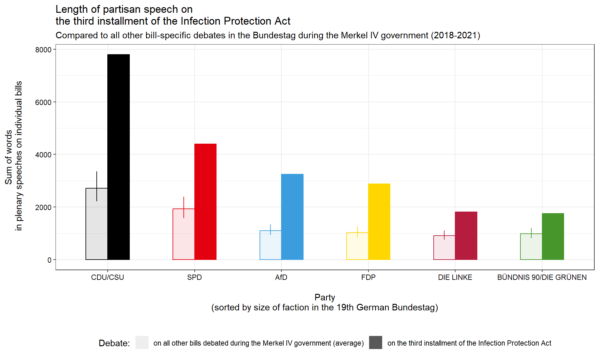
  labs(title = "Length of partisan speech on\nthe third installment of the Infection Protection Act",
       subtitle = "Compared to all other bill-specific debates in the Bundestag during the Merkel IV government (2018-2021)",
       x = " \nParty\n(sorted by size of faction in the 19th German Bundestag)\n",
       y = "Sum of words\n in plenary speeches on individual bills\n ",
       alpha = "Debate:")+
  theme_bw()+
  theme(legend.position = "bottom",
        axis.text = element_text(color = "black"))

This figure initially shows that all partisan factions in the German Bundestag spoke significantly more on the third installment of the Infection Protection Act than they spoke on the average bill during the Merkel IV government. This act indeed garnered plenary attention way above average levels.

The data also suggest that partisan speaking time is indeed roughly proportional to the seat share a party holds in the Bundestag (recall that the x-axis is sorted along this share). But interestingly, the increase of speaking time on the Third Infection Protection Act does not look really proportional. Let’s inspect the increases by party numerically.

NumberOfWordsWide <- NumberOfWords %>% 
  select(party, covid, mean) %>% 
  mutate(covid = ifelse(covid, "InfectionAct", "OtherBills")) %>% 
  pivot_wider(id_cols = party, names_from = covid, values_from = mean) %>% 
  mutate(IncreaseFactor = round(InfectionAct/OtherBills, 1)) %>% 
  arrange(desc(IncreaseFactor))
names(NumberOfWordsWide) <- c("Party", "Average words on other bills", "Words on Infection Act", "Increase Factor")
kable(NumberOfWordsWide)

This confirms the visual impression. In contrast to what the internal Bundestag rules would lead us to expect and as compared to the average bill, some parties seem to have increased their speaking time on the Infection Protection Act more than others.

The conservative CDU/CSU faction as well as two largest opposition parties, the far-right AfD and the liberal FDP, increased their number of words by almost a factor of three compared to the average bill. In contrast, MPs from the social-democratic SPD and from the two smaller opposition parties, the Left and the Greens, roughly only doubled their average amount of bill-specific speech.

Thus, the disproportional increases in plenary attention did not pit government against opposition parties but rather seem to divide parties tending to the right of the German political spectrum from those tending towards the left.

How did these partisan speakers position themselves on this Third Infection Protection Act more substantially?

To pursue this question we exploit the full-text data that ParlLawSpeech offers and build on Proksch et al (2018, LSQ) who demonstrate that the sentiment expressed in bill-specific partisan speeches reliably reveals government-opposition dynamics in plenary speeches.

In their simplest form, sentiment analyses classify texts based on their ratio of positive to negative words, drawn from a separate dictionary. For our exemplary application we use a publicly available dictionary of positive and negative terms that has been shown to map well on human impressions of German political language (Rauh 2018, JITP).

# Sentiment dictionary presented in Rauh (2018, Journal of Information Technology and Politics)
# Publically available at https://doi.org/10.7910/DVN/BKBXWD
load(here("TutorialInputs", "Rauh_SentDictionaryGerman.Rdata")) # Creates object called 'sent.dictionary'

This dictionary contains 17,330 positively and 19,750 negatively connoted German terms. To count how often these terms occur in our parliamentary speeches, we rely on the quanteda R package which offers a powerful suite of frequency-based text analysis tools, including dictionary-based approaches.

# Transform the Rauh word lists into 'dictionary' object as used by the quanteda package
# Essentially two named lists containing terms with positive (pos) and negative (neg) sentiment scores
dict <- list(pos = sent.dictionary$feature[sent.dictionary$sentiment == 1], 
             neg = sent.dictionary$feature[sent.dictionary$sentiment == -1]) %>% 
  dictionary()

We use quanteda’s core functions to tokenize each of our speeches into individual words, construct a document-frequency-matrix, in which we then count the occurrence of positive and negative terms from the sentiment dictionary.

sentiCount <- 
  corpus(speeches$text) %>% 
  tokens() %>% 
  dfm() %>% 
  dfm_lookup(dictionary = dict) %>% 
  convert(to = "data.frame")

We then calculate a sentiment score for each speech as the log-odds ratio of positive to negative words (cf. Lowe et al. 2011, Proksch et al 2018) and add this information to the speech data set.

sentiCount$score <- log((sentiCount$pos + .5)/ (sentiCount$neg +.5))
speeches$sentiment <- sentiCount$score

Finally, we mark the debate on the Third Infection Protection Act in this data and clean up some of the other group labels.

# Mark law
speeches$covid <- ifelse(speeches$procedure_ID == "19/23944/19",
                         "on the third installment of the Infection Protection Act",
                         "on all other bills debated during the Merkel IV government") %>% 
  factor(levels = c("on the third installment of the Infection Protection Act", "on all other bills debated during the Merkel IV government"))

# Order parties
speeches$party2 <- factor(speeches$party,
                          levels = c("DIE LINKE", "AfD", "BÜNDNIS 90/DIE GRÜNEN", "FDP", "SPD", "CDU/CSU"))

# Mark governing parties
speeches$gov <- ifelse(speeches$party == "CDU/CSU" | speeches$party == "SPD", "Government parties", "Opposition parties")

Now we have all the information we need in one place and can visualize the sentiment that partisan speeches expressed on the Third Infection Protection Act in comparison to all other 820 bills tabled in the German Bundestag during the Merkel IV grand-coalition government.

ggplot(speeches, aes(x = party2, y = sentiment, colour = party2, shape = covid))+
  geom_hline(yintercept = mean(speeches$sentiment, na.rm = T), linetype = "dashed")+
  stat_summary(geom = "pointrange", fun.data = mean_cl_boot, position = position_dodge(width = .5), size = .8)+
  scale_color_manual(values = c("#b61c3e", "#3c9dde", "#46962b", "#ffd600", "#E3000F", "black"), guide = "none")+
  scale_shape_manual(values = c(19, 4))+
  guides(shape = guide_legend(nrow=2,byrow=TRUE))+
  facet_grid(gov~., scales = "free_y", space = "free_y")+
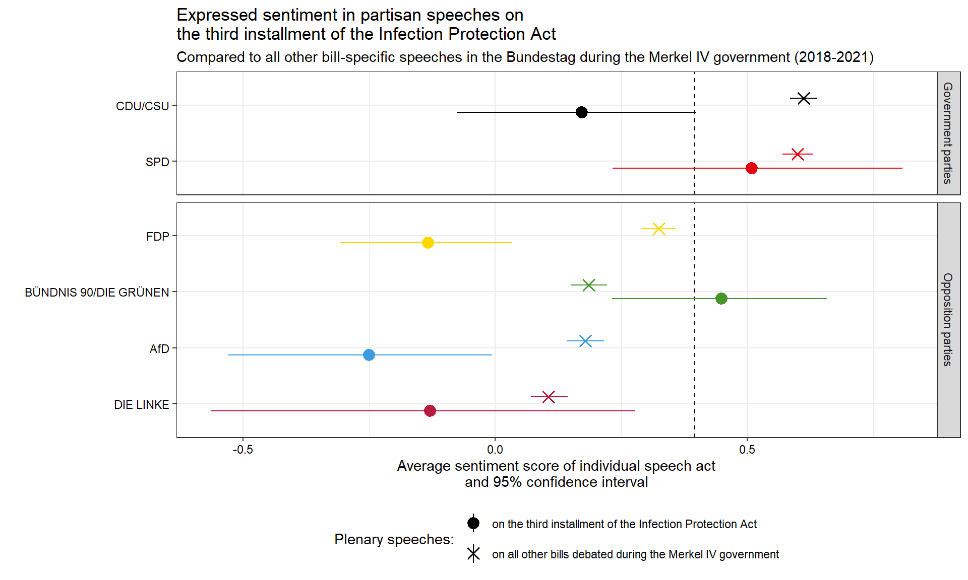
  labs(title = "Expressed sentiment in partisan speeches on\nthe third installment of the Infection Protection Act",
       subtitle = "Compared to all other bill-specific speeches in the Bundestag during the Merkel IV government (2018-2021)",
       x = " ",
       y = "Average sentiment score of individual speech act\nand 95% confidence interval",
       shape = "Plenary speeches:")+
  coord_flip()+
  theme_bw()+
  theme(legend.position = "bottom",
        legend.box="vertical",
        axis.text = element_text(color = "black"))

These data initially confirm the findings of Proksch et al 2018: The sentiment expressed in bill-specific debates clearly distinguishes government from opposition parties. The average sentiment values and their confidence intervals on bills during the Merkel IV government (marked by cross-hair symbols in the figure) clearly separate the governing CDU/CSU and SPD factions with above-average sentiment levels, from the four opposition parties with below-average sentiment score in their plenary speeches.

However, the debate on the Third Infection Protection Act does not fit this typical pattern of government-opposition dynamics. In particular, speakers from the governing CDU/CSU coalition use notably more negative language than speakers from their coalition partner SPD. And also the sentiment expressed among the opposition parties differs strongly. While MPs from the far-right AfD, the liberal FDP, and partially also from the far-left Linke express much more negative sentiment than in their usual bill-specific speeches, Green MPs express an above-average sentiment level that comes close to that expressed in speeches of social-democratic MPs from the governing coalition.

In sum, this exemplary analysis suggests that the parliamentary debate on the major German law to provide the executive with partially far-reaching counter-measures to contain Covid-19 indeed deviated from the typical dynamics in Germany’s lower chamber, but probably not along the lines that the government had hoped for: plenary attention was indeed higher but also more disproportional than on the average bills, pushing parties that expressed more negative sentiment which itself was not structured along the usual split between governing and opposition parties.

Of course, this exemplary analysis should also not be over-interpreted - the bill was ultimately accepted with votes from the governing coalition and the Greens. But it shows that analyzing and comparing bill-specific debates holds insights that go beyond the mere analysis of voting results.
From here, further analysis could dig into party-specific word-frequency patterns, or apply more advanced NLP methods of aspect-based stance detection or semantic scaling of the arguments MPs provide. So go ahead, the ParlLawSpeech data is waiting for you …